Like a car insurer, the main challenge for an options seller is to identify the best strike price based on the probability that the price will not reach that level of deviation within a certain time and to assess its value to determine if the risk taken is worth the premium received. The probability of the price reaching a certain level affects the risk that the options seller takes on. It is important to understand the historical behavior of these probabilities in order to compare the data to the current market conditions and determine the best strike price.
In this case study, we want to sell a PUT at the beginning of the week with an expiration date at the end of the week. We want to maintain a historical success probability of 80%, meaning that in 8 out of 10 instances, the price has not experienced this maximum deviation.
Starting from your initial trading idea, usually the result of other analyses, you will decide whether you want to sell a CALL or a PUT. To inform this type of decision, you can enrich your analysis by filtering the period in which you will make the transaction to see the average historical trends and perhaps discover that in that month, that particular stock tends to go down in 59% of cases, for example. In this case, the goal is to sell a PUT, thus taking a “non-bearish” position, meaning you start to profit if the price rises, or as time passes, even if the price drops slightly. (This is why it’s called “non-bearish” and not “long”)
Knowing that each filter yields a dataset of varying size and similarity to the current market conditions, we will begin a series of searches with the series filter aimed at gathering information to help us understand historical behavior. Since each applied filter changes the probabilities and the number of similar historical cases, it’s important to conduct multiple searches and extrapolate a definitive “personal” data point, perhaps by combining multiple analyses.
For each analysis, we will take a look and note down these values, as well as the number of records extracted from each search:
The MetricAlgo tool to use in this case is the Limits Analysis tool, which is part of the Historical Stats toolset.. Select the APPLE stock from the Dashboard and enter the tool where we will start to set the filters to perform the analysis. The first thing to set is the timeframe, which in this case will be set to “weekly,” and we recommend selecting only the last 20 years of the series.
The various combinations of filters and the corresponding searches that we will carry out could be:
to which we add another set of identical analyses but with an additional filter on volatility, for example, in a range of +/- 5% from the current volatility value. This way, you can compare historical results with others that are more specific to the important context of “the same volatility”.
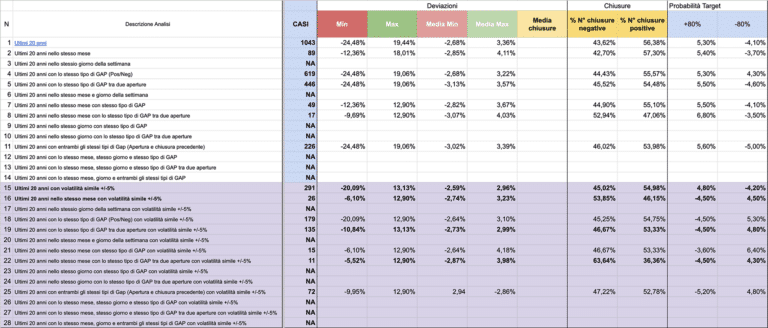
In this way, from the previous 14 analyses, we would obtain 28, with two sets differing by volatility. Here’s an example in the image:

It goes without saying that an analysis of the last 15 or 10 years will each yield another set of 28 results. Furthermore, it’s important to understand that choosing volatility as the final element of comparison is an arbitrary decision by the trader or historical data analyst, who can decide the order they prefer in their filtered investigation of the series.
Moreover, for completeness, it should be mentioned that some of these analyses do not make sense in specific time frames; for example, analyzing a weekly period while trying to filter by “day of the week” is not applicable.
Once all the analyses are performed, we can compare the data and immediately notice that adding the volatility filter excludes those periods not correlated with this metric and refines the data offered by almost one percentage point.
Since I arbitrarily consider that in a weekly timeframe, the gap between Monday’s opening and Friday’s closing is statistically insignificant, while the gap between the two openings indicates a precise trend, I have decided to make use of the 4 results highlighted in bold and to further investigate additional data starting from this basis.

After analyzing the data, starting with my bullish idea, I decided that the put sold would be at -3.5% from the current price for 5 trading days, and I sold the put for a premium of 67 euros.
The important thing for me was to identify the statistics of the deviations which, as much as the exceptional cases may scare me, I must never forget that most of the time, we are dealing with cases of normality.
In this case, the rising but not yet very high volatility made me realize that we are still in a phase of statistical normality, and for this reason, I decided to take on a final risk greater than 20%.
